SoC Integration Testing: IP-Integrated Debug and Analysis

 

One of the things I've always liked about side projects is the freedom to stop and explore a topic of interest as it comes up. One such topic that came up for me recently is IP-integrated debug and analysis instrumentation. I started thinking about this after the last post (link) which focused on exposing a higher-abstraction-level view of processor-core execution. My initial approach to doing this involved a separate bus-functional model (BFM) intended to connect to any RISC-V processor core via an interface. After my initial work on this bus-functional model that could be bolted onto a RISC-V core, two things occurred to me:

• Wouldn't it be helpful if processor cores came with this type of visibility built-in instead of as a separate bolt-on tool?
• Wouldn't SoC bring-up be simpler if more of the IPs within the SoC exposed an abstracted view of what they were doing internally instead of forcing us to squint at (nearly) meaningless signals and guess?

And, with that, I decided to take a detour to explore this a bit more. Now, it's not unheard of to create an abstracted view of an IP's operation during block-level verification. Often, external monitors that are used to reconstruct aspects of the design state, and that information is used to guide stimulus generation, or as part of correctness checking. Some amount of probing down into the design may also be done.

While this is great for block-level verification, none of this infrastructure can reasonably move forward to the SoC level. That leaves us with extremely limited visibility when trying to debug a failure at SoC level.

If debug and analysis instrumentation were embedded into the IP during its development, an abstracted view of the IP's operation would consistently be available independent of whether it's being verified at block level or whether it's part of a much larger system.

Approach

After experimenting with this a bit, I've concluded that the process of embedding debug and analysis instrumentation within an IP is actually pretty straightforward. The key goals guiding the approach are:

• Adding instrumentation must impose no overhead when the design is synthesized. 
• Exposing debug and analysis information must be optional. We don't want to slow down simulation unnecessarily if we're not even taking advantage of the debug information

When adding embedded debug and analysis instrumentation to an IP, our first step is to create a 'socket' within the IP to which we can route the lower-level signals from which we'll construct the higher-level view of the IP's operation. From a design RTL perspective, this socket is an empty module whose ports are all inputs. We instance this 'debug-socket' module in the design and connect the signals of interest to it.

Because the module contains no implementation and only accepts inputs, synthesis tools very efficiently optimize it out. This means that having the debug socket imposes no overhead on the synthesized result.

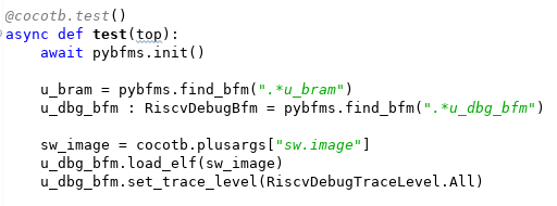
Of course, we need to plug something into the debug socket. In the example we're about to see, what we put in the socket is a Python-based bus functional model. The same thing could, of course, be done with a SystemVerilog/UVM agent as well.

Example - DMA Engine

Let's look at a simple example of adding instrumentation to an existing IP. Over the years, I've frequently used the wb_dma core from opencores.org as a learning vehicle, and when creating examples. I created my first OVM testbench around the wb_dma core, learned how to migrate to UVM with it, and have even used it in SoC-level examples. 

DMA Block Diagram

The wb_dma IP supports up to 31 DMA channels internally that all communicate with the outside world via two initiator interfaces and are controlled by a register interface. It isn't overly complex, but determining what the DMA engine is attempting to do by observing traffic on the interfaces is a real challenge!

When debugging a potential issue with the DMA, the key pieces of information to have are:

• When is a channel active? In other words, when does it have pending transfers to perform?
• When a channel is active, what is it's configuration? In other words, source/destination address, transfer size, etc.
• When is a channel actually performing transfers?

While there may be additional things we'd like to know, this is a good start.

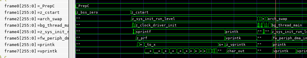
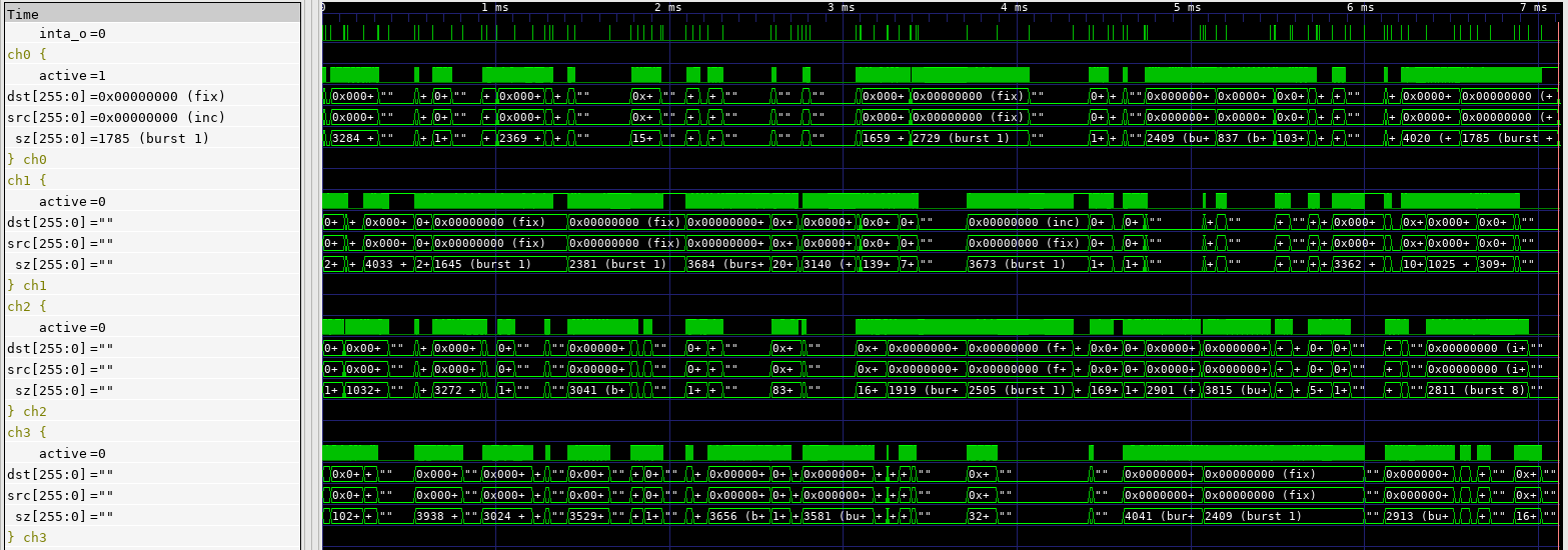
The waveform trace above shows the abstracted view of operation produced for the DMA engine. Note the groups of traces that each describe what one channel is doing. The dst, src, and sz traces describe how an active channel is configured. If the channel is inactive, these traces are blanked out. The active signal is high when the channel is actually performing transfers. Looking at the duty cycle of the active signals across simultaneously-active channels gives us a good sense for whether a given channel is being given sufficient access to the initiator interfaces. 

Let's dig into the details a bit more on how this is implemented.

DMA Debug/Analysis Socket

We first need to establish a debug/analysis "socket" -- an empty module -- that has access to all the signals we need. In the fwperiph-dma IP (a derivative of the original wb_dma project), this socket is implemented by the fwperiph_dma_debug module. 

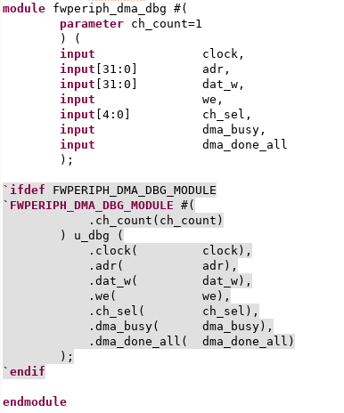
And, that's all we need. The debug/analysis socket has access to:

• Register writes (adr, dat_w, we)
• Information on which channel is active (ch_sel, dma_busy)
• Information on when a transfer completes (dma_done_all)

Note that, within the module, we have an `ifdef block allowing us to instance a module. This is the mechanism via which we insert the actual debug BFM into the design. Ideally, we would use the SystemVerilog bind construct, but this IP is designed to support a pure-Verilog flow. The `ifdef block accomplishes roughly the same thing as a type bind.

Debug/Analysis BFM

The debug/analysis BFM has two components. One is a Verilog module that translates from the low-level signals up to operations such as "write channel 2 CSR" and "transfer on channel 3 complete". This module is about 250 lines of code, much of it of low complexity. 

The other component of the BFM is the Python class that tracks the higher-level view of what channels are active, how they are configured, and ensures that the debug information exposed in signal traces is updated. The Python BFM can also provide callbacks to enable higher-level analysis in Python. The Python BFM is around 150 lines of code. 

So, in total we have ~400 lines of code dedicated to debug and analysis -- a similar amount and style to what might be present in a block-level verification environment. The difference, here, is that this same code is reusable when we move to SoC level. 

Results

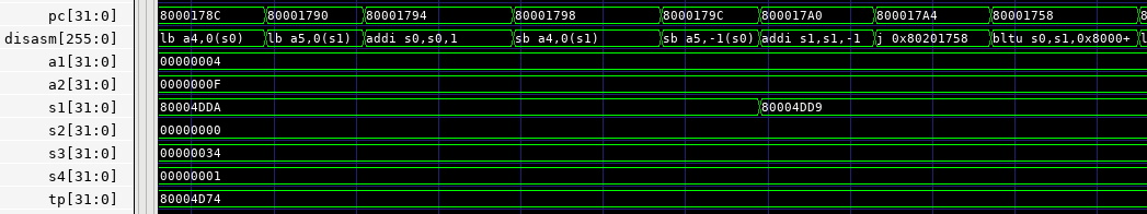
Thus far, I've mostly used the waveform-centric view provided by the DMA-controller integrated debug. Visual inspection isn't the most-efficient way to do analysis, but I've already had a couple of 'ah-ha' moments while developing some cocotb-based tests for the DMA controller. 

I was developing a full-traffic test that was intended to keep all DMA channels busy for most of the time when I saw the pattern in the image above. Notice that a transfer starts on each channel (left-hand side), and no other transfers start until all the previously-started transfers are complete (center-screen). Something similar happens on the right-hand side of the trace. Seeing this pattern graphically alerted me that my test was unintentionally waiting for all transfers to complete before starting the next batch, and thus artificially throttling activity on the DMA engine.

With the test issue corrected, the image above shows expected behavior where new transfers start while other channels are still busy.

Looking Forward

I've found the notion of IP-integrated debug and analysis instrumentation very intriguing, and early experience indicates that it's useful in practice. It's certainly true that not all IPs benefit from exposing this type of information, but my feeling is that many that contain complex, potentially-parallel, operations exposed via simple interfaces will. Examples, such as DMA engines, processor cores, and PCIe/USB/Ethernet controllers come to mind. And, think how nice it would be to have IP with this capability built-in!

In this blog post, we've looked at the information exposed via the waveform trace. This is great to debug the IP's behavior -- while it's being verified on its own or during SoC bring-up. At the SoC level, the higher-level information exposed by at the Python level may be even more important. As we move to SoC level, we become increasingly interested in validation -- specifically, confirming that we have configured the various IPs in the design to support the intended use, but not over-configured them and, thus, incurred excess implementation costs. My feeling is that the information exposed at the Python level can help to derive performance metrics to help answer these questions.

This has been a fun detour, and I plan to continue exploring it in the future -- especially, how it can enable higher-level analysis in Python. But, now it's time to look at how we can bring the embedded-software and hardware (Python)  portions of our SoC testbench closer together. Look for that in the new few weeks.

References

• wb_dma IP (original Wishbone DMA IP) -- https://opencores.org/projects/wb_dma
• fwperiph-dma IP (Modified DMA IP) -- https://github.com/Featherweight-IP/fwperiph-dma

Disclaimer

The views and opinions expressed above are solely those of the author and do not represent those of my employer or any other party.

SoC Integration Testing: Higher-Level Software Debug Visibility

Debug is a key task in any development task. Whether debugging application-level software or a hardware design, a key to productive debug is getting a higher-level view of what is happening in the design. Blindly stepping around in source code or staring at low-level waveforms is rarely a productive approach to debugging. Debug-log messages provide a high-level view of what's happening in an software application, allowing us to better target what source we actually inspect. Testbench logging, coupled with a transaction-level view of interface activity, provides us that higher-level view when verifying IP-level designs. Much of this is lacking when it comes to verifying SoC integration.

Challenges at SoC Level

We face a few unique challenges when doing SoC-integration testing. Software (okay, really firmware) is an integral part of our test environment, but that software is running really really slowly since it is running at RTL-simulation speeds. That makes using debug messages impractical, since simulating execution of the code to produce messages makes our test software run excruciatingly slowly. In addition, the types of issues we are likely to find -- especially early on -- are not at the application-level anyway. 

Processor simulation models often provide some form of execution trace, such as ARM's Tarmac file, which provides us a window into what's happening in the software. The downsides, here, are that we end up having to manually correlate low-level execution with higher-level application execution and what's happening in the waveform. There are also some very nice commercial integrated hardware/software debug tools that dramatically simplify the task of debugging software at the source level and correlating that with what's happening in the hardware design -- well worth checking out if you have access.

RISC-V VIP

At IP level, it's common to use Verification IP to relate the signal-level view of implementation with the more-abstract level we use when developing tests and debugging. It's highly desirable, of course, to be able to use Verification IP across multiple IPs and projects. This requires the existence of a common protocol that VIP can be developed to comprehend. 

If we want VIP that exposes a higher-level view of a processor's execution, we'll need just such a common protocol to interpret. The good news is that there is such a protocol for the RISC-V architecture: the RISC-V Formal Interface (RVFI). As its name suggests, the RISC-V Formal Interface was developed to enable a variety of RISC-V cores to be formally verified using the same library of formal properties. Using the RVFI as our common 'protocol' to understand the execution of a RISC-V processor enables us to develop a Verification IP that supports any processor that implements the RVFI.

RISC-V Debug BFM

The RISC-V Debug BFM is part of the PyBfms project and, like the other Bus-Functional Models within the project, implements low-level behavior in Verilog and higher-level behavior in Python. Like other PyBfms models, the RISC-V Debug BFM works nicely with cocotb testbench environments.

Instruction-Level Trace

Like other BFMs, the Verilog side of the RISC-V Debug BFM contains various mechanics for converting the input signals to a higher-level instruction trace. Consequently, the signals that expose the higher-level view of software execution are collected in a sub-module of the BFM instance.

The image above shows the elements within the debug BFM. The ctxt scope contains the higher-abstraction view of software execution, while the regs scope inside it contains the register state.

The first level of debug visibility that we receive is at the instruction level. The RISC-V Debug BFM exposes a simple disassembly of the executed instructions on the disasm signal within the ctxt scope. Note that you need to set the trace format to ASCII or String (depending on your waveform viewer) to see the disassembly. 

C-Level Execution Trace

Seeing instruction execution and register values is useful, but still leaves us looking at software execution at a very low level. This is very limiting, and especially so if we're attempting to understand the execution of software that we didn't write -- booting of an RTOS, for example. 

Fortunately, our BFM is connected to Python and there's a readily-available library (pyelftools) for accessing symbols and other information from the software image being executed by the processor core.

The code snippet above shows our testbench obtaining the path to the ELF file from cocotb, and passing this to the RISC-V Debug BFM. Now, what can we do with a stream of instruction-execution events and an ELF file? How about reconstructing the call stack?

The screenshot above shows the call stack of the Zephyr OS booting and running a short user program. If we need to debug a design failure, we can always correlate it to where the software was when the failure occurred. 

The screenshot above covers approximately 2ms of simulation time. At this scale, the signal-level details at the top of the waveform view are incomprehensible. The instruction-level view in the middle are difficult to interpret, though perhaps you could infer something from the register values. However, the C-level execution view at the bottom is still largely legible. Even when function execution is too brief to enable the function name to be legible, sweeping the cursor makes the execution flow easy to follow.

Current Status and Looking Forward

The RISC-V Debug BFM is still early in its development cycle, with additional opportunities for new features (stay tuned!) and a need for increased stability and documentation. That said, feel free to have a look and consider whether having access to the features described above would improve your SoC bring-up experience.

Looking forward in this series of blog posts, we'll be looking next at some of the additional things we can do with the information and events collected by the RISC-V Debug BFM. Among other things, these will allow us to more tightly connect the execution of our Python-based testbench with the execution of our test software.

Finally, the process of creating the RISC-V BFM has me thinking about the possibilities when assembling an SoC from IPs with integrated higher-level debug. What if not only the processor core but also the DMA engine, internal accelerators, and external communication IPs were all able to show a high-level view of what they were doing? It would certainly give the SoC integrator a better view of what was happening, and even facilitate discussions with the IP developer. How would IP with integrated high-level debug improve your SoC bring-up experience?

Disclaimer

The views and opinions expressed above are solely those of the author and do not represent those of my employer or any other party.

Python Verification Stimulus and Coverage: Constraints

Over the past few blog posts, we've looked at:

• The fundamentals of modeling stimulus and functional coverage in Python
• Modeling verification data types in Python
• Modeling and capturing functional coverage in Python
• Making use of captured coverage data

In this post, we will look at how to model constraints in Python using the PyVSC library. Several libraries that I'm familiar with (mostly C++) provide a way to embed constraints using an embedded domains-specific language. I've felt some discontent with the way that this is done because it's fairly different from what we're familiar with in languages that treat constraints as first-class language constructs.  Specifically, in C++, constraints are often modeled as lists of comma-separated expressions, and not as blocks of statements the way a first-class language would model them. This means that constraints that would normally be grouped in a block need to be split up into multiple blocks. And, when constraints are combined, they become difficult to read. One of my motivations in examining Python's support for embedded domain-specific languages was to see if Python offered a better approach. My feeling is that it most definitely does, and I hope you agree.

The examples in this post come from the PyVSC documentation. The latest version is always directly available on readthedocs.io.

Constraint Blocks

Constraint blocks in PyVSC are special class methods that are decorated with a constraint Python decorator. The presence of the constraint decorator causes PyVSC to see treat these methods, not as a regular Python method, but as an element to construct a constraint expression model. Here's a simple example:

@vsc.randobj
 class my_base_s(object):

     def __init__(self):
         self.a = vsc.rand_bit_t(8)
         self.b = vsc.rand_bit_t(8)

     @vsc.constraint
     def ab_c(self):
        self.a < self.b

PyVSC calls the methods marked as constraints once during the class-elaboration process and creates an internal model of the constraint statements captured in these constraint blocks. It also replaces the method with a class field that has special properties. More on that later.

By overloading operators (such as "<"), PyVSC is able to get an expression tree that can be given to the Boolector SMT solver that does all the heavy-lifting of constraint solving for PyVSC. 

As in SystemVerilog, constraint blocks are considered "virtual". In other words, having a constraint in a sub-class with the same name as a constraint in a base class causes the base-class constraint to be replaced with the sub-class constraint. 

@vsc.randobj
class my_base_s(object):

    def __init__(self):
        self.a = vsc.rand_bit_t(8)
        self.b = vsc.rand_bit_t(8)
        self.c = vsc.rand_bit_t(8)
        self.d = vsc.rand_bit_t(8)

    @vsc.constraint
    def ab_c(self):
       self.a < self.b

@vsc.randobj
class my_ext_s(my_base_s):

    def __init__(self):
        super().__init__()
        self.a = vsc.rand_bit_t(8)
        self.b = vsc.rand_bit_t(8)
        self.c = vsc.rand_bit_t(8)
        self.d = vsc.rand_bit_t(8)

    @vsc.constraint
    def ab_c(self):
       self.a > self.b

In the example above, the ab_c constraint in the sub-class my_ext_s overrides the ab_c constraint in the base class my_base_s. The effect is that instances of my_ext_s will enforce the relationship (a > b) instead of the base-class relationship (b < a).

Constraint Expressions

PyVSC supports specifying constraints using the familiar set of expression constructs we're all used to using: <, >, ==, !=, etc. The one set of operators that do not behave as you would expect in Python are the logical ones: and, or, etc. Python doesn't allow overriding these logical operators, unlike other operators. Consequently, we use bit-wise operators instead. 

with my_i.randomize_with() as it:
    it.a_small() | it.a_large()

In the example above, a_small and a_large are boolean constraints. Normally, in Python, we would combine these using or. In a PyVSC constraint, we use | instead.

There are two special expressions to be aware of that can be used in constraints: the 'in' expression and part select. Both of these are frequently used in Python, and both can be used in constraints with PyVSC.

@vsc.randobj
class my_s(object):

    def __init__(self):
        self.a = vsc.rand_bit_t(8)
        self.b = vsc.rand_bit_t(8)
        self.c = vsc.rand_bit_t(8)
        self.d = vsc.rand_bit_t(8)

    @vsc.constraint
    def ab_c(self):

       self.a in vsc.rangelist(1, 2, [4,8])
       self.c != 0
       self.d != 0

       self.c < self.d
       self.b in vsc.rangelist([self.c,self.d])

The 'in' expression operates on a PyVSC-type field on the left-hand side and a PyVSC rangelist on the right-hand side. A rangelist can contain individual values and ranges of values. A rangelist can contain both constant expressions, such as the literals shown in the first rangelist, and expressions involving other PyVSC variables.

Python provides array-slicing expressions, and PyVSC reuses these to implement bit-slicing of scalar fields.

@vsc.randobj
class my_s(object):

    def __init__(self):
        self.a = vsc.rand_bit_t(32)
        self.b = vsc.rand_bit_t(32)

    @vsc.constraint
    def ab_c(self):

        self.a[7:3] != 0
        self.a[4] != 0

In this example, the part-select operator is used to ensure that certain bits and bit-ranges within the 'a' field are non-zero.

Constraint Statements

Statements pose two additional challenges when developing an embedded domain-specific language: often keywords are already in use by the host language (and cannot be overloaded), and languages often don't provide easy way to overload statement blocks. Here, Python definitely has some benefits. Now, not surprisingly, Python doesn't allow overloading of built-in statements.But, it does provide an easy-to-use way of creating scopes that can be used to capture block statements. 

PyVSC provides three constraint statements. If/else and Implies are block statements, while the 'unique' constraint is not.

Python's mechanism for introducing a block of statements is the 'with' statement. When combined with a user-defined object, the 'with' statement allows a library writer to comprehend statement blocks. Here is an example of an if/else constraint:

@vsc.randobj
class my_s(object):

    def __init__(self):
        self.a = vsc.rand_bit_t(8)
        self.b = vsc.rand_bit_t(8)
        self.c = vsc.rand_bit_t(8)
        self.d = vsc.rand_bit_t(8)

    @vsc.constraint
    def ab_c(self):

        self.a == 5

        with vsc.if_then(self.a == 1):
            self.b == 1
        with vsc.else_if(self.a == 2):
            self.b == 2

The if_then class is used to form the 'if' branch of an if/else statement. Additional 'else-if' branches can be added on with the 'else_if' class. The final 'else' case is described with the 'else_then' class. 

The implies constraint is similar, since 'implies' applies to a constraint block:

class my_s(object):

    def __init__(self):
        super().__init__()
        self.a = vsc.rand_bit_t(8)
        self.b = vsc.rand_bit_t(8)
        self.c = vsc.rand_bit_t(8)

    @vsc.constraint
    def ab_c(self):

        with vsc.implies(self.a == 1):
            self.b == 1

Finally, the 'unique' constraint ensures that the specified terms have a unique value:

@vsc.rand_obj
class my_s(object):

    def __init__(self):
        self.a = vsc.rand_bit_t(32)
        self.b = vsc.rand_bit_t(32)
        self.c = vsc.rand_bit_t(32)
        self.d = vsc.rand_bit_t(32)

    @vsc.constraint
    def ab_c(self):
        vsc.unique(self.a, self.b, self.c, self.d)

Customizing Declared Constraints

In general, we want to specify most of our constraints as part of the class hierarchy. However, there are quite a few cases where we need to customize things a bit when we randomize the class. PyVSC provides two capabilities to enable this: in-line constraints, and constraint mode.

In-line constraints allow us to add extra constraints that are specific to a randomization. To use this capability, use the 'randomize_with' call instead the the 'randomize' call as shown below:

@vsc.randobj
class my_base_s(object):

    def __init__(self):
        self.a = vsc.rand_bit_t(8)
        self.b = vsc.rand_bit_t(8)

    @vsc.constraint
    def ab_c(self):
       self.a < self.b

item = my_base_s()
for i in range(10):
   with item.randomize_with() as it:
     it.a == i

The example above ensures that 'a' increments 0..9 across 10 randomization calls. Note that the fields of the class can either be referenced via the handle that is being randomized (item) or via a special variable created by the 'with' block.

Constraint-mode allows entire constraint blocks to be turned on and off. Error-injection is one use-case for this feature. 

 @vsc.randobj
 class my_item(object):

     def __init__(self):
         self.a = vsc.rand_bit_t(8)
         self.b = vsc.rand_bit_t(8)

     @vsc.constraint
     def valid_ab_c(self):
        self.a < self.b

item = my_item()
# Always generate valid values
for i in range(10):
   item.randomize()

item.valid_ab_c.constraint_mode(False)

# Allow invalid values
for i in range(10):
   item.randomize()

As shown in the example above, the first 10 randomizations have all constraints enabled. The next 10 randomizations have the 'valid_ab_c' constraint block disabled, allowing invalid values to be produced.

Next Steps

Over the past few posts, we've looked at the key features and capabilities of PyVSC, a Python library for modeling constraints and functional coverage for verification. I would encourage you to use PyVSC, report bugs, and suggest enhancements. PyVSC is, of course, an open-source project, so contributions in the form of pull requests for bug fixes, documentation updates, and enhancements are always welcome as well.

For the last few months (pretty close to a year, actually) I've been really focused on hardware-centric functional verification infrastructure, with a focus on Python. I'm thinking it's time to get back to focusing a bit more on firmware development and embedded-software verification. There have been some interesting developments in this space, recently, which have the potential to enable significant changes in the way we develop and verify firmware and other low-level software. Look for more on that soon. Until then, stay safe and keep learning!

 

Disclaimer
The views and opinions expressed above are solely those of the author and do not represent those of my employer or any other party.

Python Verification: Working with Coverage Data

Before jumping into this week's post, I wanted to offer a bit of an apology to my readers. I recently realized that, despite being a Google property, Blogger only notifies authors of comments for moderation if the author has specifically registered a 'moderator' email with the site. So, apologies to those of you that have commented on posts directly on the Blogger site and watched those comments hang out in limbo indefinitely. I should now receive notifications of new comments.

In my last post, we looked at modeling and sampling functional coverage in Python using the Python Verification Stimulus and Coverage (PyVSC). In that post, I showed how a textual coverage report could be generated to the console by calling an API. But, there is much more that we want to do with functional coverage data. The key question is: how do we store and manipulate it?

Storing Coverage Data

There are two big motivations for storing coverage data. The first is that we often wish to aggregate coverage across a large number of tool runs. In order to do that, we need a way to persist the coverage data collected by each individual tool run. The second is that we want to run analysis on the collected and aggregated coverage data. We want a way to browse through the data interactively, and create nice-looking reports and charts.

Standard Coverage Models

Storing coverage data isn't much different than storing any other data. The first big question to answer is whether there is a standard way of of representing the data, or whether we need to invent one. While I've certainly had fun in the past inventing new formats for representing and storing data, considering all the requirements and designing in appropriate features to represent all the key features of a given type of data is a time consuming problem. Certainly something that should be undertaken as a last resort.

The good news is that there are several existing formats for representing coverage. The bad news is that the vast majority are focused on representing code coverage data (eg Coburtura), not functional coverage data. That said, there is one industry standard for representing functional coverage and code coverage: Accellera Unified Coverage Interoperability Standard. 

While the  UCIS defines several things, it doesn't define a standard database format. That said, what it does define is very useful. Specifically it defines:

• A data model for representing functional coverage, code coverage, and assertion coverage
• A C-style API for accessing and modifying this data model
• An XML interchange format to assist in moving data from one database implementation to another. In a pinch, the XML interchange format can even be used as a very simplistic database.

Design is tough, so it's almost always most efficient to make use of the work of a committee of smart and capable people instead of starting over. UCIS is certainly not perfect. There are some "bugs" in the spec, and some internal inconsistencies. That said, it's far better than starting with a blank sheet of paper. The next challenge was adapting UCIS to Python.

PyUCIS Library

Much of my work recently has been in Python, so I wanted a way to work with the UCIS data model in Python. The PyUCIS library is a pure-Python library for working with the UCIS data model. A block diagram of the architecture is shown below. 

Front-End API

The core of the PyUCIS library is an implementation of the UCIS API. Remember that the API defined by the UCIS is a C-style API, while Python is much more object-oriented. I initially decided to implement just an object-oriented version of the UCIS API, but then realized that reusing existing code snippets written in C would be much harder without an implementation of the C-style API. Fortunately, building a C-style compatibility API on top of the object-oriented one was fairly straightforward.

Backend

The PyUCIS library uses a back-end to store the data being accessed via the front-end API. The PyUCIS library currently implements two back ends: an in-memory back-end, and an interface to existing C-API implementations of the UCIS API.

The in-memory back-end stores coverage data in Python data structures. While it's not possible to persist the data model directly, the contents can be saved to and restored from the XML interchange format specified by the UCIS.

The C-library back-end uses the Python ctypes library to call the UCIS C API as implemented by a tool-specific shared library. This allows PyUCIS to access data in databases implemented by tools that support UCIS.

While PyUCIS doesn't currently implement its own native database for storing coverage data, it's likely that it will in the future. Fortunately, Python provides an SQLite database as part of the core interpreter installation. Stay tuned here.

Built-in Apps

The final part of the PyUCIS library are a set of built-in apps. These are used to perform simple manipulations on the coverage data and create outputs. Currently, PyUCIS only contains one built-in app: reading and writing the UCIS XML interchange format. That said, there are a couple planned on the roadmap:

• A merge app to combine data from multiple UCIS data models
• A report app to produce a textual or HTML coverage report

PyUCIS Apps

The top layer of the PyUCIS architecture diagram are external applications that use the PyUCIS API. At the moment, there is only one and it's a proof of concept. PyUCIS Viewer is a Python Qt5-based GUI for viewing coverage data.

While the viewer is certainly primitive (and incomplete) at the moment, hopefully this provides some ideas for what can be done with the data accessed via the PyUCIS API.

Next Steps

PyUCIS is a pretty early-stage tool. I'm using it to save coverage data from the PyVSC library, and to produce some simple text coverage reports, but there's still quite a bit to do. As always, if you'd like to contribute to this or other projects, I'd welcome the help. 

In the next post, I'll return the Python Verification Stimulus and Coverage (PyVSC) library to look at modeling constrained-random stimulus. Until then, stay safe!

Disclaimer

The views and opinions expressed above are solely those of the author and do not represent those of my employer or any other party.